


[Page 305]Abstract: The drought recorded in Helaman 11 is probably the only dated, climate-related event in the entire Book of Mormon that could have left a “signature” detectable over 2,000 years after it occurred. Typical methods to detect this kind of event using dendrochronology (the study of tree rings) or sediment cores from lake beds either do not go back far enough in time or are not of high enough resolution to detect the event described in Helaman 11. However, over the last 15 to 20 years, various researchers have turned to analyzing stalagmites collected from caves to reproduce the precipitation history of a given area. These analysis methods are now producing results approaching the 1–year resolution of dendrochronology, with 2 sigma (95%) dating accuracies on the order of a decade. There is an ongoing debate with regard to where the events in the Book of Mormon took place. One of the proposed areas is Mesoamerica, specifically in southern Mexico and Guatemala. This paper will test the hypothesis that the drought described in the Book of Helaman took place in Mesoamerica using the results of precipitation histories derived from the analysis of three stalagmites compared to determine if there is evidence that a drought took place in the expected time frame and with the expected duration.
The Book of Mormon records that the prophet Nephi, son of Helaman, asked God to cause a famine in the land with the hope that it would end the destruction and wickedness caused by a war with the Gaddianton robbers1 (Helaman 11:2, 10). This event is unique in the Book of Mormon because it may be the only recorded event that can be dated within an accuracy of a few years and that might have left an [Page 306]imprint or signature that could be detected today, over 2,000 years after it took place. This famine had the following characteristics:
- Three- to 3.5-year duration. It began during the 73rd year of the reign of the judges (Helaman 11:2–5), 19 “Book of Mormon years” before the birth of Christ (3 Nephi 1:4– 13). It ended during the 76th year of the reign of the judges (Helaman 11:17), 16 “Book of Mormon years” before the birth of Christ.
- Involved a relatively large geographic area that extended outside of Nephite lands (Helaman 11:6).
- Caused primarily by a lack of rain, not some other reason like war, plant diseases, or locusts, for example (Helaman 11:6, 13, 17).
- Severe enough that it stopped the war, and “they did perish by the thousands in the more wicked parts of the land” (Helaman 11:6).
Dating this event in terms of Book of Mormon chronology depends on what year Christ was born. There are differing opinions on this subject, but the proposed dates are generally within a range of about 4–5 years. A few of the proposed dates are described below:
- Doctrine and Covenants 20:1 indicates a date of 6 April 1 BC for the birth of Christ. (There is no year 0, so if he were born on 6 April 1 BC, he would have been 1 year old on 6 April 1 AD, and his birth could also be specified as being 0 AD)
- Spackman argues, based on historical evidence, that Lehi must have left Jerusalem sometime between the spring of 588 and the spring of 587 BC2 He also accepts scriptural and historical sources that indicate Jesus Christ was born in the spring of 5 BC, but his claim is that the only way to fit 600 years from time Lehi left Jerusalem to this birth of Christ is to assume the Nephites used a 12–moon lunar calendar so their years were shorter than present-day solar years.
- Pratt compares the evidence for several dates that have [Page 307]been proposed for Christ’s birth.3 He argues, based on some of the same historical evidence as Spackman concerning events before and after the Biblical account of the birth of Christ, that Christ was born around the time of the Passover, about 6–9 April, 1 BC
- Humphries compares the Biblical account and Persian customs/traditions with historic astronomical and other evidence4 to propose that the star of Bethlehem was a comet documented in Chinese records and that the date of the birth of Christ was sometime during the period 13–27 April 5 BC, which also coincides with Passover of that year.
- Dunn indicates, “Jesus himself is generally reckoned to have been born some time before the death of Herod the Great in 4 BCe. A date between 6 BCe and 4 BCe would accord with such historical information as Matthew’s birth narrative assumes (Matthew 2.16) and with the tradition of Luke 3.23 that Jesus was ‘about thirty years age’ in the fifteenth year of Tiberius Caesar (Luke 3.1), reckoned as 27 or 28 CE.”5
Many other sources, both Latter-day Saint and non-Latter-day Saint, could be cited, but all sources the author is aware of fall within the range of years defined by the sources cited above. This range produces a corresponding range for the years when the drought described in Helaman would have occurred. All that is necessary is to determine whether or not this range of years for the drought event overlaps the range of years of drought events in geographic areas of interest defined from other sources.
These proposed dates for the birth of Christ generate a range of years when the beginning of the drought could have taken place. If the spring of 6 BC is used as the date Christ was born and solar years are assumed, the beginning of the drought could have been as early as the spring of 25 BC If the spring of 1 BC is used as the date of the birth of Christ and lunar years are assumed, the beginning of the drought (converted to current the modern calendar) could have been as late as the fall of 20 BC [Page 308](using 12×19 lunar cycles and a lunar cycle = 29.53 days2). This drought can therefore be described as starting any time from 25 BC through 20 BC inclusive, having a duration of 3 to 3.5 years and being severe enough that most crops could not grow because of the lack of precipitation.
To resolve the confusion of the calendar schemes (i.e., BCE/CE, BC/ AD), the remainder of this paper will use the convention of +/- AD to indicate years, since this designation is familiar to most people and avoids the issue of the missing year 0 in the BC/AD convention, especially when doing associated math. So, the drought can be described as starting as early as the spring of -24 AD and as late as the fall of -19 AD.
Detecting a drought as short as 3 to 3.5 years over 2,000 years ago presents difficult challenges. The method used to reconstruct the precipitation history needs a resolution on the order of half of the duration of the event being sampled. This means the time between samples of the precipitation history must be about 1.75 years or less. Any approach having a width between samples that is much larger than this value might not detect the event, or even if it does, it would only provide an extremely coarse measure of its duration. Of course, the approach for constructing the precipitation history of some geographic area would also require a way of determining the date or year associated with any given sample and to estimate the accuracy of that association.
Many people are familiar with dendrochronology — the study of tree rings to reconstruct the precipitation history of a given area. The width of the rings can be used to estimate the amount of precipitation by correlating the widths of the rings with known precipitation records in modern times. The earliest portions of the ring width “patterns” from modern trees are then correlated with the most recent patterns of older trees whose life overlapped the modern trees. As long as trees can be identified in a given area whose lives continuously overlapped backward in time, this method can provide a continuous estimate of the precipitation history that extends back before precipitation records were kept. The date associated with each “sample” or tree ring of this precipitation is determined by simply counting the number of tree rings to the desired year in the past. This method of constructing a precipitation history satisfies the requirements for detecting the event in the Book of Helaman since it has a resolution that is ~1 year per sample and can be dated to an accuracy of ~1 year.
[Page 309]One proposed location for the events of the Book of Mormon is the Mesoamerican area, described in great detail by Sorenson.6 But with regard to the drought described in Helaman and a proposed setting of Mesoamerica, dendochronology is of no use because the oldest tree ring chronologies of the Mesoamerican region do not cover the period of interest, -24 to -19 AD. The oldest dated tree ring in this region comes from central Mexico and begins in AD 771.7 However, over the last 15–20 years, researchers have been developing methods that have resolutions high enough and dating accurate enough to begin to identify drought events with the characteristics specified in the account recorded in Helaman.8 In addition, these methods have been used to generate precipitation histories for the Mesoamerican region.9 This paper will test the hypothesis that the drought described in the Book of Helaman took place in the geographic area known as Mesoamerica using the results of precipitation histories derived from these new sources and methods.
[Page 310]High Resolution Methods of Estimating Precipitation
One of the postulated theories for the demise of the Mayan and other Mesoamerican civilizations has been that it was caused by prolonged droughts on the order of many decades.10 This has motivated researchers to develop methods for reconstructing the precipitation history of Mesoamerica.11 Another motivation has been the study of historical climate patterns for the Mesoamerican region as they relate to present climate change and the effect of prolonged conditions like El Niño on weather patterns.12
To achieve both high resolution and accurate dating, many researchers have turned to the use of speleothems (cave deposits), such as stalagmites growing in caves in the region of interest.13 The resolution of the precipitation history obtained from stalagmites is dependent on several factors. One important factor is the rate of growth of the stalagmite.14 A comparatively short stalagmite that grew over a particular time would have a poorer resolution than a much longer stalagmite that grew over the same period. Another factor affecting resolution is the method used to sample the growth patterns of the stalagmite along its length.15 For example, curent methods require the stalagmite to be split along its axis. Holes are drilled along the central axis of the stalagmite to provide material for various chemical measurements. The resolution of these methods depends on the width of the drill bit and the spacing between drilled holes. The material removed from a majority of the holes is used to reconstruct the precipitation history, while the material from a smaller subset of holes provides dates (with an associated date accuracy) at the corresponding points along the stalagmite’s axis.16 These “date” measurements are used to create a “date model” to estimate the date at any arbitrary point in the precipitation history.17
These invasive methods and a non-invasive method using light for reconstructing a high-resolution precipitation history from stalagmites [Page 311]are briefly described below. At this point, the reader may want to skip forward to the “Is Mesoamerica ‘the land?’ Published Research Results” section if the following details are not of interest — they are rather technical. However, they are provided to help understand the published results. For in-depth investigation on the subject of using speleothems to reconstruct precipitation history, the textbook Speleothem Science: From Process to Past Environments is available.18
Proxy Measurements for Precipitation
Luminescence
The luminescence method19 uses ultraviolet light to illuminate a narrow (~2 millimeter) region on the central axis of one of the split halves of the stalagmite while recording the luminescence (color) pattern with a camera scanned along its entire length. These patterns are produced by organic acids shown to be dependent on the amount of vegetation produced by the soil in the vicinity of the cave where the stalagmite was formed. Since the amount of vegetation correlates with the amount of precipitation, this luminescence pattern can be used as a proxy for rainfall. Low luminescence (less organic acids) corresponds to periods of lower precipitation, while higher luminescence (more organic acids) corresponds to times with higher precipitation. Since this method is non-invasive (it does not involve drilling), its resolution is dependent only on the rate of growth of the stalagmite. Drilling is still required to produce material for estimating dates/ages along the axis of the stalagmite, but these “age” drill holes are typically spaced much further apart than those drilled for other methods.
[Page 312]Oxygen Isotope Concentration Ratio
The oxygen isotope concentration ratio method20 measures the concentration of two stable isotopes of oxygen in powders produced from drilling holes at periodic points along the central axis of a split half of the stalagmite. The measured concentration ratio, 18O/16O, is used to determine δ18O (read delta-O-18, which is a direct proxy for precipitation) by comparing it with the oxygen concentration ratio of a standard, such as Vienna Standard Mean Ocean Water (VSMOW) or Pee Dee Belamnite (PDB), or Vienna Pee Dee Belamnite (VPDB). δ18O is normally expressed in parts per thousand (0/00 VSMOW, or PDB or VPDB depending on which standard is used). To ensure the δ18O values derived from measurements are a valid proxy for rainfall, several measurements at the growth end of the stalagmite are compared with modern, recorded rainfall records in the region where the cave/ stalagmite was located.
δ18O is a proxy for rainfall in the stalagmites studied in Meso America primarily due to preferential evaporation rates of the lighter 16O in the nearby ocean. Rain falling on land areas close to the ocean therefore has a higher concentration of 16O. During drier conditions with less rainfall over the area of the cave, fewer molecules containing 16O are present, causing the concentration ratio of minerals in the stalagmite that contain oxygen, hence δ18O, to rise. During wetter conditions with more rainfall, more molecules containing 16O become incorporated into the minerals in the stalagmite, causing the concentration ratio and δ18O to decrease.
Carbon Isotope Concentration Ratio
The carbon isotope concentration ratio method21 measures the concentration of two stable isotopes of carbon in powders produced from drilling holes at periodic points along the central axis of one of the halves of the stalagmite. The measured concentration ratio, 13C/12C, is used to determine δ13C (read delta-C-13, which is an indirect proxy [Page 313]for precipitation) by comparing it with the carbon concentration ratio of a standard such as Pee Dee Belamnite (PDB) or Vienna Pee Dee Belamnite (VPDB). δ13C is normally expressed in parts per thousand (0/00 PDB or VPDB, depending on what standard is used).
δ13C is an indirect proxy for rainfall in stalagmites because most plants increase the levels of 12CO2 in the soil, which percolates to the caves where the stalagmites are growing and participates in formation of the calcium carbonate (CaCO3) that makes up the stalagmite. Higher levels of rainfall create more plant material, which increases the level of 12CO2 in the soil. But a higher amount of 12C decreases the concentration ratio, 13C/12C, used to determine δ13C. In drier periods, there is less plant growth and lower levels of 12CO2 available to form CaCO3, which has the effect of increasing the carbon concentration ratio and δ13C.
Determining the Age of Measurements
The method of choice for dating stalagmites appears to be uranium thorium and is commonly referred to as “U-series” dating, although carbon-14 dating has also been used.22 Even lead-210, with a short half-life of 22.2 years, has been used for recent growth portions of stalagmites. Typically, powder from a few of the holes drilled along the central axis of one of the halves of the stalagmite are used to determine dates as a function of distance along the collected stalagmite. These dates are used to generate an age model that can be applied to the delta-isotope measurements that are also a function of distance along the axis of the stalagmite. The age model may be as simple as linear interpolation between dated points or may employ the use of a MATLAB program to perform more sophisticated date estimation techniques. Date accuracies obtained by researchers within the last five years or so have been specified to be on the order of +/- 10 years for samples on the order of 2,000 years old. Accuracies specified in the remainder of this document will be 2-sigma Gaussian values, which correspond to a 95.45% probability that the true values are within two standard deviations (sigmas) of the indicated mean value.
Is Mesoamerica “The Land?” Published Research Results
To date, there are four published papers documenting the analysis of three different stalagmites using techniques with sufficient resolution and that cover the period of interest over 2,000 years ago in the [Page 314]Mesoamerican area. Two of the stalagmites were collected from two different caves in Belize. The third was collected in the mountains of southern Mexico. Their locations are shown in Figure 1. Oxygen and carbon isotope measurements along with the associated U-series ages can be downloaded from the NOAA National Climatic Data Center23 for each stalagmite from Yok Balum Cave24 and the Macal Chasm25 in Belize, and from Juxtlahuaca Cave26 in Mexico. The Macal Chasm stalagmite was recently re-analyzed. This new analysis produced higher resolution data and has an age model27 more clearly defined than that in the original published paper.28 They are described below in the date order they were collected.
Macal Chasm (Belize)
The stalagmite obtained from Macal Chasm was designated MC01 by the researchers who conducted the analysis and reported the results.29 It was collected some time in late 1995 or early 1996 and is 92 centimeters in length. Several methods were used to reconstruct the precipitation history recorded in MC01. The results of only two have resolutions high enough to meet the requirements specified above to detect the event recorded in Helaman. The authors refer to these methods as “petrographic examination”30 and “ultraviolet-stimulated luminescence,” or UVL.31
Petrographic analysis examines the crystalline structure of the stalagmite to identify transitional boundaries between layers. There are two important types of boundaries that are of interest. As explained by the authors,
Type E surfaces show signs of layer erosion and are associated with increased water flow, while Type L surfaces have layers [Page 315]that rapidly thin away from the apex and are associated with reduced water flow and lessened CaCO3 deposition.32
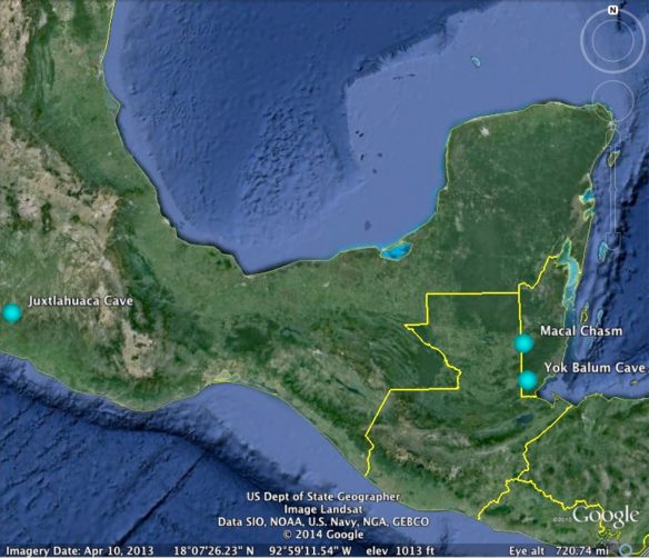
Figure 1. Map of cave locations in Mesoamerica where stalagmites were collected.
No Type E boundaries were identified in MC01, while 15 Type L boundaries were found during the period ~4,700 years Before Present (BP), where BP is 1995. Five of these Type L boundary layers coincide with the Nephite Book of Mormon time span and are specified in Table 1.
The authors of the most recent analysis33 indicate the resolution of the luminescence data has a median pixel interval of .066 mm that corresponds to a median 0.38 years of growth per pixel. This is an improvement from the original analysis34 which was about .5–3 years per pixel, based on a pixel interval of ~.18 mm and estimated stalagmite growth rates of .069 – .402 mm/year.
| [Page 316]Depth | Age (Years Before 1995) | Date | 95% Confidence Interval | Petrographic Boundary Type |
| 22.8 cm | 1,585 | 410 AD | +/- 347 yrs | L-type |
| 28.7 cm | 2,020 | -25 AD | +/- 367 yrs | L-type |
| 29.1 cm | 2,045 | -50 AD | +/- 365 yrs | L-type |
| 33.0 cm | 2,320 | -325 AD | +/- 336 yrs | L-type |
| 36.0 cm | 2,500 | -505 AD | +/- 322 yrs | L-type |
Table 1. List of Type-L boundaries that Overlap the
Nephite Book of Mormon Time Span (Akers, et. al., 2016).
This resolution satisfies the requirements for detecting the drought described in Helaman. However, the confidence intervals of the age model are quite large due to the low uranium concentrations present in MC01. Because of these large confidence intervals, the authors identify somewhat long periods where all precipitation proxies indicate below average rainfall. They call each of these periods a “major dry event” or MDE. An MDE is defined as
a multi-decadal period with sustained values of δ18O and δ13C substantially higher (>10/00 and >30/00, respectively) than preceding and following values that coincide with UVL values substantially lower (>100 lower) than preceding and following values. Additionally, an MDE will include petrographic evidence of significant dryness in the form of a Type L boundary. The thinning layers associated with Type L boundaries are physical evidence of reduced stalagmite growth and support the conclusion that higher δ18O and δ13C values coincide with lower UVL indicate drier conditions.35
They also indicate that the “Type L boundaries associated with the MDEs are always found at the end of an MDE; that is, the Type L boundary caps the stalagmite zone with high stable isotope values and low UVL values.”36 Once the MDEs were identified, the authors correlate the associated times with other published results to show that, at least on a multi-decadal time scale, there is agreement between those results.37
In a similar way, we will correlate and compare the Type L boundary events in Table 1, the luminescence data for MC01 with the data from [Page 317]other published high-resolution results, and the drought event described in Helaman 11 in a summary section at the end of this paper.
Juxtlahuaca Cave (Mexico)
A stalagmite was collected from deep (~800 meters from the cave entrance) within Juxtlahuaca Cave in May 2010 and designated JX-6 by the researchers who performed the analysis.38 The much longer distance of the stalagmite from the cave entrance is a factor that distinguishes it from the other stalagmites in Belize considered in this article, which were both near their respective cave entrances. This fact significantly affected the age model and date accuracies for JX-6. The age model created by the researchers is based on 20 U-series measurements over a 1,041-mm span of the 1,115-mm long stalagmite. The oldest sample dates to around 4,000 years before the time of collection, but discontinuous growth was evident until about 2,400 years before the time of collection, so the published results span only the most recent 2,400 years.
The reconstructed precipitation history is based on δ18O measurements made from micro milling at 1-mm intervals, which corresponds to an average ~3-year resolution. These measurements are available on the NOAA website.39 δ13C measurements were made but not published. The researchers used the results to compare and assess the impact of droughts on the inhabitants of the Basin of Mexico and particularly the civilization based at Teotihuacán.
The researchers calibrated the measured oxygen isotope precipitation history by using rainfall records from the Tacubaya climate station near Mexico City from 1880 to 2010 and showed correlation between rainfall patterns in Mexico City and the cave location.40 The researchers’ analysis indicated a variable time lag for the rainfall water to make its way through ~160 meters of bedrock (epikarst) above the cave to JX-6. While observations of drip rates in the cavern where JX-6 was located indicated seasonality and provided evidence of some fairly direct conduits for the water from the surface to the JX-6 location, most of the water took anywhere from 4 to 14.5 years to make its way to the JX-6 [Page 318]location. The absolute values of the published correlation coefficients of this analysis are all greater than or equal to .80 for each year in this range, with the peak correlation being .89 at a lag of nine years.41 Based on this calibration analysis, the researchers also produced a five-year running average dataset of rainfall versus time shown shifted backward in time by the nine-year delay when compared to the raw data set.
The underlying assumption is that this delay is constant over the life of the stalagmite, which, in all likelihood, cannot be proven one way or another. It would seem that over time, mineral-laden waters percolating through bedrock could tend to precipitate out in some places and plug up water channels through the bedrock. This could cause an increased overall delay as time goes on, which could cause the delay observed in modern times to be greater than the delay 2,000 years ago. At the same time, water could dissolve minerals in the epikarst and open up water channels through bedrock. This process obviously occurs, or the cave containing the stalagmite would not have formed in the first place. Which of these processes contributes more over the passage of time is anyone’s guess. Personal correspondence with the lead researcher42 indicates an innumerable number of water channels through the epikarst, each with a different delay, and that a simple average [Page 319]time shift was all that could be done, given what was known about the epikarst, but the true effect of the epikarst is much more complicated than a simple single time delay would imply.43
Yok Balum Cave (Belize)
The stalagmite from the Yok Balum cave in Belize was collected in June 2006 from a spot approximately 50 meters from the cave entrance; it is 607 mm in length and was designated YOK-1. Due to discontinuities and complex growth patterns in the lower (oldest) region, the researchers published results only for the upper (most recent) 415 mm of the stalagmite.44 This region was dated to a period from 40 BC to the year of collection in 2006, so this time span barely covers the event in Helaman. The age model is based on 40 U-series measurements on the upper 444 mm of the stalagmite.
Reconstructed precipitation histories based on δ18O and δ13C measurements were published and are available from NOAA.45 More than 4,200 stable isotope measurements were made on the upper 415 mm of YOK-1. The sample holes were milled at 0.1 mm intervals, resulting in a resolution from .01 to 3.68 years. Of the three stalagmites reviewed in this paper, the reconstructed histories of YOK-1 have both high resolution and the best accuracies. However, the authors indicate a major divergence between the δ18O and δ13/C measurements during the most recent 150 years of the datasets and that the δ18O measurements are not consistent with the known historical precipitation records for this area in Belize, but the δ13C measurements are consistent with those records. The researchers could not explain the reason for this divergence in the δ18O measurements but indicated that the δ18O measurements before this time are valid.
Correlating the Proxy Precipitation Histories
Figure 2 displays the various proxy precipitation histories measured from each stalagmite that overlap some portion of the -600 AD to +425 AD time [Page 320]of Nephite civilization. All graphs are oriented so that increasing dryness is in the direction toward the top of the page. Increasing wetness is therefore in the direction toward the bottom of the page. Various horizontal solid and/or dashed lines have been drawn across each graph to specify various averages and/or drought thresholds. These are labeled to the right of each graph in the corresponding legend. These thresholds are unique to each stalagmite and measurement type and reflect what the corresponding researchers specified as the definition of a drought or what would correspond to average precipitation. Determining the width or duration of a drought is somewhat problematic because each duration depends on the threshold used with a particular data set. And comparing those durations across multiple data sets using different thresholds is somewhat an “apples to oranges” comparison. The best that can be done in this regard is to determine if the various observed droughts are “consistent” with the account in Helaman. The first step will be to correlate the possible droughts across each proxy history and identify those that have commonality between the various histories recorded in each stalagmite. This will provide assurance that the same event was recorded by each stalagmite and was not due to some local phenomenon or something unique to a particular cave. The second step will involve focusing down to the period of interest recorded in the account in Heleman, around -20 AD, and making similar comparisons there.
There are two graphs from the Juxtlahauca Cave. The first at the top is the graph of the raw measured δ18O values versus time. A value of 8.0 is the average for this graph. There are two dashed lines above this average. The upper line is labeled as “2-σ From Average” and represents the threshold of drought defined for this data set. There are four “error bars” just under the horizontal time axis at the top of this graph that define the 95% confidence intervals at the peak of each drought at about -50, -92, -195, and 310 AD. Corresponding vertical grey bars extend down across the next two graphs to correlate these droughts from the Juxtlahuaca graphs with the Macal Chasm graph.
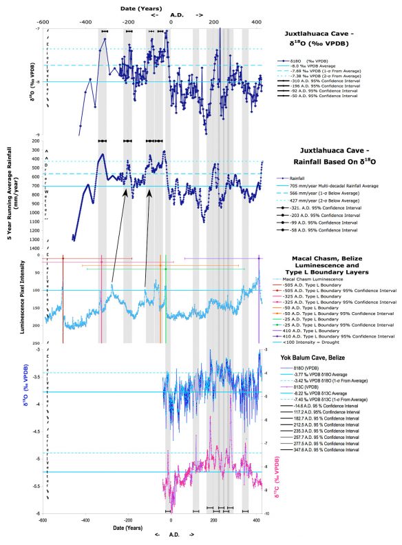
Figure 2. Comparison of precipitation proxy data for the Nephite period (Lachniet, et al., Akers, et al., Kennett, et al., NCDC).
The second Juxtlahuaca graph is a five-year running average rainfall over the same time span as the oxygen isotope ratio graph. As explained previously, the researchers calibrated the raw data in the first graph, shifting it by nine years into the past and smoothed the result by calculating the five-year running average shown in the second graph. This averaging process, by definition, will broaden/lengthen any defined drought peaks by about five years in this graph when compared to the raw oxygen isotope ratio graph. The vertical grey bars that define the [Page 321]drought confidence intervals line up with the peaks in this second graph, rather than those in the raw oxygen isotope ratio graph because it is the calibrated, and presumably more accurate, result. The reader should keep in mind that these confidence intervals are not durations of droughts. They are intervals of time that define when the actual peak of [Page 322]the drought seen in the graph could have occurred. In other words, one could grab the peak and stretch or pull the peak to the left or to the right within the defined confidence interval. There are also four confidence intervals above the peaks in this running average rainfall graph. They are wider than the corresponding confidence intervals in the raw oxygen isotope ratio graphs to take into account the subtraction of the average nine-year lag. This nine-year lag is really a random variable with a standard deviation that affects the resulting variance associated with each peak.46
This visual “correlation” approach is used because the peaks and events of the third graph for the Macal Chasm, as previously specified in Table 1, have very large confidence intervals and cannot be reliably used for determining the dates of events unless they are compared and correlated with other, more accurately dated events from the other two stalagmites. Only these four droughts are referenced from the Juxtlahuaca stalagmite because only the Juxtlahuaca precipitation proxy histories overlap the Macal Chasm for the period before 40 AD, when the Yok Balum record begins. All other drought events later than -40 AD are referenced using the Yok Balum record because it has the highest [Page 323]reported accuracy of the three stalagmites. The error bars defining those 95% confidence intervals are therefore just above the horizontal time axis at the bottom of the Yok Balum graph and the grey bars extend upward across all the other graphs of the other stalagmites.
The Macal Chasm graph contains the Type L boundary layer events in addition to the luminescence precipitation proxy history. These boundary events appear as vertical lines at the indicated date. It is clear that the left-most and right-most of the four Juxtlahuaca drought events at -325 AD and -50 AD correlate very well with corresponding Type L boundary layers and luminescence peaks in the Macal Chasm record. The other two drought events in between these two dates do not appear to have corresponding peaks in the Macal Chasm record. But it is significant that the Macal Chasm luminescence graph does show exactly two other peaks that would each qualify as a drought at values of less than or equal to 100 pixel intensity during this time span. They could correspond to these two Juxlahuaca drought events because they are well within the +/-300-year 95% confidence intervals associated with the Macal Chasm data. This is illustrated by the two arrows pointing from the Macal Chasm peaks to the corresponding Juxlahuaca peaks. Between these two drought events in both stalagmite records is a single, pronounced, “wet” period or a “dip” around 175 AD. This provides solid evidence that the two stalagmites are recording the same events, despite the large confidence intervals specified for the Macal Chasm record.
The Book of Mormon is silent with regard to events that might be related to climate around the time of any of these four drought events. They may have been weak in severity or not important enough to mention in Mormon’s abridgement. Or perhaps the reason the Helaman account is the only mention of a drought over a 1,000-year history was that it was the only one specifically requested by a prophet of God, that it came to pass as requested, and that it ended as requested, understandably an important lesson to teach and record in a religious record.
The Yok Balum stalagmite record is used as a reference to correlate with drought events for the other two stalagmites for the time span later than 40 AD, when the Yok Balum record begins. It is readily apparent that the carbon isotope ratio graph is much less “noisy” than the oxygen isotope ratio graph, with very well defined peaks that define potential drought events. The carbon isotope ratio is used here as the basis for defining potential drought events using the 1-sigma above average threshold at -7.4 0/00 VPDB (right vertical axis) as long as there is a corresponding peak, above the 2-sigma threshold, in the Yok Balum [Page 324]oxygen isotope ratio graph that is within the 95% confidence interval associated with the carbon isotope ratio peak. The Yok Balum oxygen isotope scale is defined by the left vertical axis of the graph.
There are eight possible drought events about -15, 117, 183, 213, 235, 258, 277, and 347 AD that meet the defined criteria. Of these, the only possible drought event that correlates with the other two stalagmite records is the one at -15 AD. The only peaks less than the 100-pixel intensity drought threshold present in the Macal Chasm graph are those at -15 AD and 410 AD. Both these peaks also have an associated Type L boundary. The 410 AD peak appears to be present only in the Juxtlahuaca Rainfall graph because of the nine-year left shift from the calibration process and the five-year averaging. It would also appear in the top raw data plot if the horizontal axis would have been extended another 15 years or so. But a peak is not present in the Yok Balum carbon isotope ratio graph at this time and yet is present in the Yok Balum oxygen isotope graph.
It is interesting to note, however, that even the Macal Chasm graph indicates drier conditions beginning around 180 AD, which coincides with clear peaks in both Yok Balum isotope ratio graphs and the Juxlahuaca graphs. And it appears there may have been multiple successive droughts or consistently drier than normal years that spanned nearly 100 years until around 280 AD. The Book of Mormon narrative just prior to and around 183 AD is very brief. However, sometime between 111 AD and 201 AD, there were some people who revolted from Christ’s church and became Lamanites. It is pure speculation, but could this long span of below-normal precipitation have been a contributing, underlying factor of this revolt?
Figure 3 “zooms in” to the time span from -120 to 40 AD to provide a closer look at the details of this single drought event that correlates across all the precipitation histories of the three stalagmites and compares it to what is known about the drought described in Helaman 11. In these graphs, the center point of the drought is defined using the width of the drought event. The width of the drought event for each stalagmite proxy record is defined to be the center point between the two points that cross the corresponding threshold for each stalagmite/data type graph. These widths are annotated in the legend for each graph.
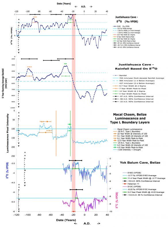
Figure 3. Comparison of precipitation proxy data for the Helaman 11 period (Lachniet, et al., Akers, et al., Kennett, et al., NCDC).
The width of the Juxtlahuaca oxygen isotope ratio plot is about 10.6 years, and for the Juxtlahuaca rainfall plot it is about 14 years. The difference of 3.4 years between the drought event widths measured between the two graphs is not surprising because the five-year running average process will broaden all peaks. This stalagmite was also deep within a cave, where the drip water was estimated to take anywhere from [Page 325]4 to 14.5 years (with an average of 9 years) to reach the stalagmite. The 3.5-year drought described in Helaman 11 could therefore appear as an event in the oxygen isotope ratio graph that was 7.5 to 18.0 years in duration or, if the average is used, a duration of 12.5 years. This 10.6- year drought duration is consistent with the conditions that formed the stalagmite and the account in Helaman 11.
[Page 326]The Macal Chasm drought event is about 6.5 years in duration or about double the duration of the event described in Helaman 11. If the “peak-to-peak” definition of the drought is used, the duration drops to 4.9 years. It is also interesting to note that the drought in the Juxtlahuaca and the Macal Chasm graphs also appear to have the same shape, with distinct peaks near the beginning and the end of the drought.
The “noisy” Yok Balum oxygen isotope ratio graph has a width of 11.4 years, while the Yok Balum carbon isotope ratio graph has a peak width of 3.2 years. This last graph has a width highly consistent with the duration of the drought described in Helaman 11. But the two isotope records for this stalagmite don’t seem to be consistent with regard to the duration of the drought.
The drought durations as measured using the various defined thresholds indicate a drought sometime between 3.2 and 11.4 years in duration, excluding the Juxtlahuaca rainfall width, which is lengthened by the five-year averaging. This compares with the account in Helaman 11 of 3.0 to 3.5 years. This exercise illustrates the difficulty in attempting to determine drought event durations and comparing them between different stalagmites using a variety of data types and their corresponding drought thresholds. There is certainly consistent evidence that the drought was less than about one decade, and very likely fewer than 6.5 years in duration, if the noisy Yok Balum oxygen isotope results are removed.
Similar to Figure 2, the 2-sigma or 95% confidence intervals are shown above each drought event (peak) for the Juxlahuaca and Yok Balum stalagmites, although in this case the mid-point of the confidence interval coincides with the middle of the drought defined by the threshold crossings of the drought peak rather than the year corresponding to the maximum peak value. The Macal Chasm confidence intervals are not shown in Figure 3 because they would simply be lines that span the entire width of the graph without providing any additional information. They can be seen in Figure 2. The period that defines the range of possible drought mid-points from the Helaman 11 account is represented by the light red vertical column that spans across all graphs. The most important result of this graph and this paper is that this time span derived from the Helaman 11 account intersects all 95% confidence intervals at the only time when all these 95% confidence intervals overlap. A five-year shift in either direction would have missed intersection with one or more confidence intervals in the Juxtlahuaco or Yok Balum graphs. Even the Macal Chasm drought with the corresponding Type L boundary layer at [Page 327]-25 AD is very close (~5 to 7 years) to the expected time frame despite the associated, large (+/- 367 years) 95% confidence interval.
Conclusion
It is simply remarkable that dating analysis methods applied to stalagmites can now be used to estimate:
- A drought occurred just over 2,000 years ago in Mesoamerica.
- This drought happened within a few years of when the Book of Mormon account says it should have happened, based on estimates from multiple proxy precipitation records from three different stalagmites in the Mesoamerican area.
- To the extent that a rough duration of this drought can be measured with the available proxy data and defined thresholds, they indicate a drought duration of somewhere between 3.2 to 11.4 years, a range that includes the 3- to 3.5-year duration described in the Book of Mormon.
Whereas there may be other places in the North/South American continents where droughts occurred during the same time frame, based on these results, the Mesoamerican area cannot be excluded as a candidate for a place where the events in the Book of Mormon occurred. The evidence from these stalagmites can now be added to a continually increasing body of evidence that points to Mesoamerica as the setting for the Book of Mormon.
Addendum
With respect to the possibility that the Helaman 11 drought event took place in the present-day United States, somewhere east of the Mississippi River, there is evidence against that hypothesis. To date, the author has found [Page 328]one stalagmite with nearly the required resolution for the period of interest a little over 2,000 years ago in the eastern United States. It was collected from the DeSoto Caverns in northern Alabama in 2008. The analysis, presented in a master’s thesis, indicates that the time from -72 AD to +28 AD was one of the wettest 100-year periods in the previous 1,500 years.47 This 100-year period is shown in Figure 4 by the darker grey-colored bar.
The analysis explains that the time series used in the plots were generated by the ARAND Time Series Analysis Software, but the time series values were not included in the thesis, other than in plots. The δ18O and δ13C measurements were included in the thesis at 0.1-mm intervals along with a table of dated samples. The author contacted Mr. Aldridge to obtain the time series, but he indicated that the hard drive where his data was kept was destroyed in hurricane Harvey in 2017. So the author constructed a plot by estimating the time series from the table of dated samples and the isotope measurements. The author believes it is adequate to provide some conclusions.
The plots in Figure 4 show the measurements for δ18O (left Y axis) and δ13C (right Y axis) over a 1,550-year span from -1500 to 50 AD for the DeSoto Cavern stalagmite. The 100-year period centered around -22 AD from -72 to 28 AD includes one of the two wettest periods during this 1,550-year time span as indicated by the more negative excursions from a ~2,000 year average equal to -3.0 +/- .5 for δ18O and shown by the top horizontal line passing through the upper plot. The short-term δ18O average over the 100-year period centered at -22 AD is -3.45. This is .94 sigmas below average/”normal” on the “wet” side of average. The long-term average δ13C value over a ~2,000-year period is -6.8 +/- 1.2 is shown by the bottom horizontal line. The short-term δ13C average over the same 100-year period, centered at 22 AD, is 8.28. This is 1.2 sigmas below average/”normal” on the “wet” side of average. The 2-sigma date accuracy for this short term, 100-year time, is 46 years. The measurement samples in this region of the stalagmite are spaced about every 2.8 years, possibly somewhat less during periods when the stalagmite was rapidly growing. This resolution is about 1 year longer than desired, but is high enough to detect a drought event as short as 3.5 years with one or two samples.
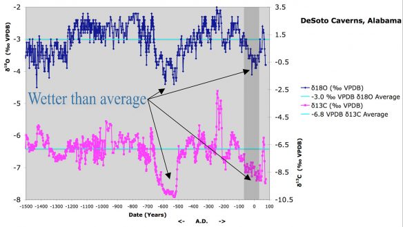
Figure 4. Precipitation proxy data for the DeSoto Cavern stalagmite (Aldridge).
[Page 329]These results indicate that it is unlikely that a drought occurred anywhere near northern Alabama within +/- 50 years of the time the drought described in the Book of Mormon occurred for the following specific reasons:
- The δ18O direct proxy for rainfall indicates significantly higher precipitation (rainfall) than average within +/- 50 years of the expected drought time frame.
- The δ13C indirect proxy for rainfall indicates significantly higher precipitation (plant growth) than average within +/- 50 years of the expected drought time frame.
- The measurement resolution is high enough (<2.8 years) that it is not likely that a 3.5-year drought event would have been “missed.” There should have been at least one and possibly two sample(s) indicating a drought. Instead, over this 100-year period, there are only 5 samples (out of 36 samples) of δ18O that barely achieve the expected average level of -3.0 (-3.0, -3.0, -2.9, -2.8, -2.8). There are no δ13C samples that achieve the long-term average of -6.8, let alone indicate any kind of drought during this relatively short, 100-year period.
- The 100-year period was selected because the 2-sigma date accuracies associated with these measurements are just less than 50 years. If the center of this interval at -22 AD is really up to +/-46 years from -22 AD (the 2-sigma accuracy specified above) because of date estimation error, the previous three statements are still true (to the significance of 2-sigma accuracy) because [Page 330]the results still include the time of the expected drought event at -22 AD Also, it should be noted, if this short-term interval is reduced by half to +/- 25 years, the results indicate even higher precipitation over this shorter time interval.
Conclusion: The data produced by the DeSoto Cavern stalagmite do not support the hypothesis that the drought event described in Helaman 11 in the Book of Mormon occurred anywhere in the vicinity of the DeSoto Caverns in northeastern Alabama. In addition to most of Alabama, this vicinity would likely include adjacent areas of northern Mississippi, northern Georgia, and central Tennessee, since regional precipitation patterns in this area are very likely to be highly correlated.
Go here to see the 18 thoughts on ““Let There Be a Famine in the Land”” or to comment on it.